

Introduction
Healthcare systems play a pivotal role in enhancing people’s health and wellbeing. In the 1950s, South Korea was one of the poorest nations globally, but has since emerged as one of the top 10 economies. Central to this transformation are robust, government-driven policies. With the enactment of the National Health Insurance (NHI) Act in 1963, 97% of the population was mandatorily enrolled in NHI by 1989, while the remaining 3% received healthcare benefits via the tax-funded Medical Aid program1-4. South Korea’s healthcare system, known for low medical costs and high accessibility, has substantially contributed to reduced mortality and morbidity5. However, social issues, including low birth, population ageing, and slow economic growth, raise concerns about the sustainability of healthcare financing, challenges faced by many developed countries5,6.
Globally, end-stage kidney disease (ESKD) is among the most costly chronic conditions. Renal replacement therapies, such as dialysis and kidney transplantation, are vital for sustaining the lives of those with ESKD. In South Korea, NHI covers approximately 60% of medical costs7 and ensures access to necessary healthcare services by regulating medical fees through government price controls8,9. Despite this, ESKD treatment requires sustained, intensive resource use, often imposing a dual burden of severely diminished quality of life and substantial household financial strain on those affected9,10. To alleviate this, the government has introduced supplementary policies, including fixed-cost treatment programs, disability registration, financial discounts for low-income households, and special healthcare cost support. Similarly, other developed countries operate specialised systems to support people with ESKD11,12. However, evaluations of health equity among those with ESKD based on geographic disparities remain limited, particularly regarding rural–urban differences, an underexplored area in many countries.
Definitions and classifications of ‘urban’ and ‘rural’ vary across regions and countries13-15. Nevertheless, disparities in health services accessibility and outcomes between urban and rural areas have become pressing global health policy issues15-21. Rural areas often face challenges such as limited transportation and infrastructure, fewer economic opportunities, and restricted access to healthcare facilities, resulting in geographic inequities in health services accessibility and household financial equity. For severe conditions requiring prolonged treatment, significant portions of household income may be allocated to out-of-pocket (OOP) expenditure, increasing the risk of financial hardship and, in some cases, forcing households to forgo healthcare services. This exacerbates health outcomes. While South Korea has implemented policies to address these challenges, evaluating these measures from diverse perspectives is essential. Identifying successful policies can motivate further improvements, and recognising shortcomings can guide reforms.
This study explores several key questions:
- Do urban and rural individuals with ESKD differ in health status and healthcare service utilisation?
- Is there a disparity in healthcare expenditure between urban and rural areas?
- How do these differences impact household financial situations?
- What household characteristics are associated with higher risks of catastrophic health expenditure (CHE)?
Using 7 years of data from the Korean Health Panel (KHP), this study aims to compare health status, health services accessibility, household finances, and financial burdens including CHE between urban and rural individuals with ESKD. The hypotheses are as follows:
- Individuals in rural areas have poorer health status than their urban counterparts.
- Rural areas face disadvantages in health services accessibility.
- Household financial conditions are worse in rural areas.
- Rural households bear greater burdens from poverty, impoverishment, and CHE prevalence.
The findings are expected to contribute to the development of universal and inclusive healthcare policies by capturing the unique health-related needs of rural areas, supporting their sustainable development.
Methods
Study design
This study utilises a mixed-methods design, combining both cross-sectional and longitudinal panel data analyses. To address potential sampling biases, all analyses used weighted populations.
Data source
The KHP is a representative dataset of South Koreans, designed to assess healthcare utilisation patterns and guide national healthcare policy directions. It is collected and managed by the NHI Service and the Korea Institute for Health and Social Affairs (KIHASA). This panel was established through the first round of data collection from 2008 to 2018, using a proportional two-stage stratified cluster sampling method to extract a sample of approximately 8000 households and their members22. Each year, trained surveyors collected data on the sociodemographic characteristics of households and their members, as well as information on financial and healthcare service utilisation, chronic diseases, and OOP expenditure. Supplementary surveys were conducted with adult panel participants aged 19 years and above to gather data on over 500 variables, including health behaviours, psychological status, and other factors. Panel participants’ illness diagnoses have been recorded using International Classification of Diseases (ICD) codes since 2012. The present study utilises data spanning 2012–2018 (a 7-year period).
To ensure accurate data on healthcare use and financial status, panel participants were required to record their healthcare use, income, and expenditure in specially designed health ledgers. The data management authorities (KIHASA) verified the quality of these records by cross-referencing them with original health insurance data, and after validation they were deemed reliable.
Observations associated with end-stage kidney disease
The total number of adult data observations from 2012 to 2018 was 97,134. Among these, 421 observations were identified as being associated with ESKD (n × years), with the annual number of ESKD individuals ranging from 49 to 68, resulting in a total of 105 unique ESKD individuals (ICD-10 code N18.6). The prevalence of ESKD per 1000 KHP individuals per year ranged from 3.97 to 4.70, and the weighted prevalence ranged from 3.58 to 3.99 (Fig1).
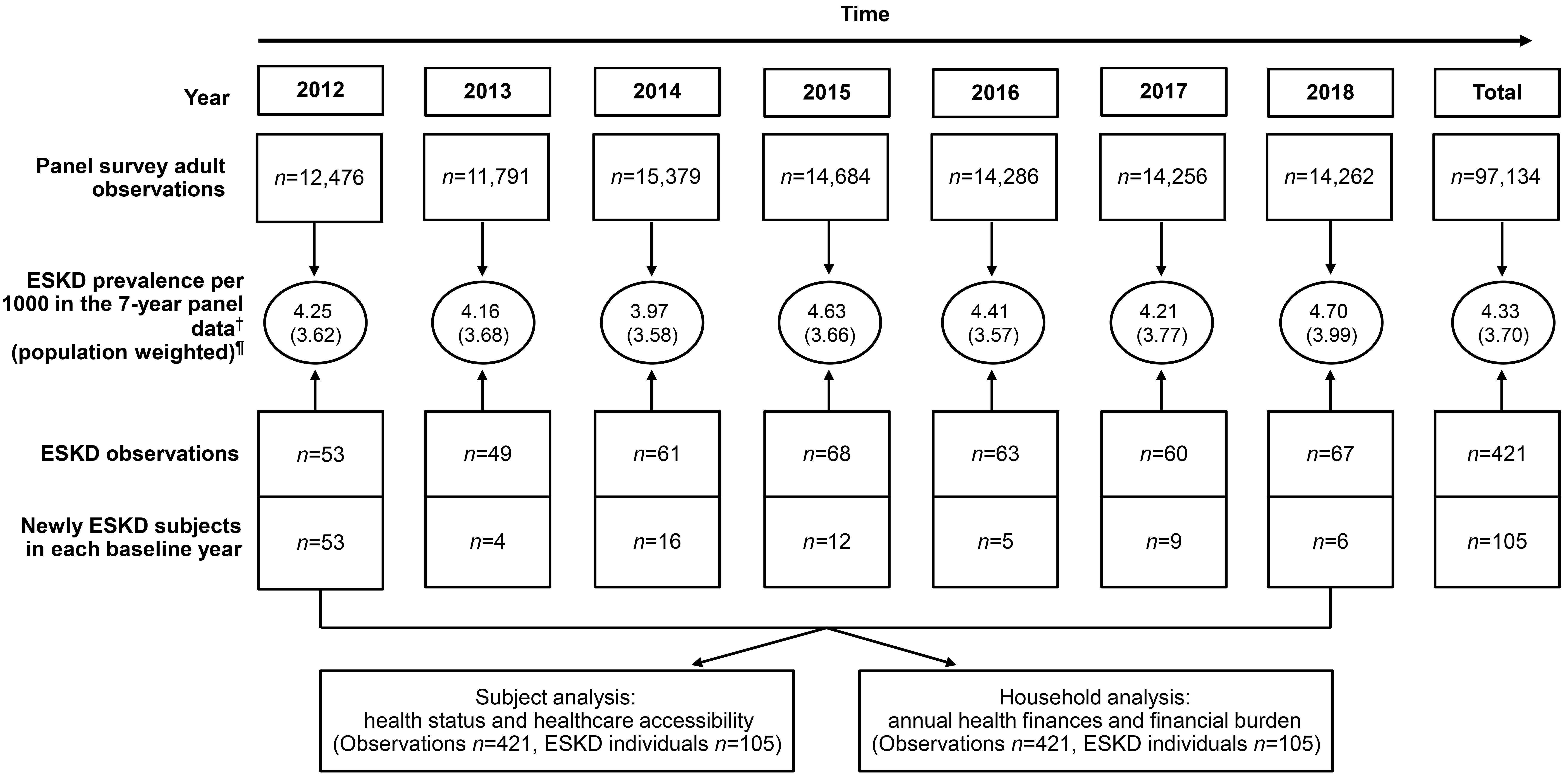 Figure 1: End-stage kidney disease (ESKD) in South Korea: annual observations, prevalence, and analysis units, 2012–2018. †(ESKD observations per year ÷ total observations per year) × 1000. ¶(ESKD observations per year within the population ÷ total observations per year within the population) × 1000.
Variables
Urban and rural areas
This study utilised urban–rural classification as the major independent variable. In South Korea, the smallest administrative units for place of residence are dong, eup, and myeon. Dong refers to urban administrative units, while eup and myeon are typically considered rural areas, with population thresholds of approximately 20,000. Accordingly, participants whose addresses were in dong were classified as urban, whereas those in eup or myeon were classified as rural15.
Sociodemographic characteristics
This study analysed variables including survey year, age, gender (man or woman), age at ESKD diagnosis, number of household members, marital status (having a spouse: yes or no), economic activity (yes or no), health insurance type (special assistance or NHI), kidney disability (yes or no), other disabilities (yes or no), receiving one or more healthcare benefits (yes or no), and household income quintiles. These variables were also used as control variables in the panel analysis model.
The special assistance category for health insurance includes individuals eligible for Medical Aid, those in the second-lowest income group, and individuals qualifying for special exceptions under provisions for rare and incurable diseases. These individuals receive comprehensive healthcare coverage, providing additional treatment cost reductions beyond the universal coverage of the NHI.
‘Kidney disability’ refers to individuals who underwent dialysis for more than 3 months, or kidney transplantation, and were registered as legally disabled under the disability registration law. Other disabilities refer to individuals with disabilities other than kidney disability, registered under one of the 15 recognised disability types.
The ‘one or more healthcare benefits’ category refers to individuals receiving healthcare benefits from the government due to being registered under special assistance, kidney disability, or other disabilities.
In the KHP, household income quintiles were adjusted for household size by dividing total income from labour and assets by the square root of the number of household members. Observations were then classified into five quintiles, ranging from the fifth quintile (highest) to the first quintile (lowest).
Health status indicators
This study used number of comorbidities, self-reported health status, and perceived satisfaction with ESKD medications as proxy variables. The number of comorbidities represents the total number of chronic diseases diagnosed by a physician within a survey year. Self-reported health reflects individuals’ assessments of their current health status; the scale was reversed to range from 5 (very good) to 1 (very poor). Perceived satisfaction with ESKD medications indicates the level of satisfaction with medications for ESKD; the scores were also reversed to range from 5 (very good) to 1 (very poor).
Health services accessibility indicators
This study assessed annual health services accessibility through the following variables: emergency room visits (yes or no), inpatient utilisation (yes or no), outpatient visits (yes or no), unmet healthcare needs (yes or no). The first three indicators were based on actual medical records, while unmet healthcare needs reflected self-reported assessment.
Annual household finances indicators
Annual household income
Annual household income refers to the total sum of labour income and income from assets within a household.
Capacity to pay
The author calculated household capacity to pay based on the method proposed by Xu (2005)23. This refers to the amount a household can pay after household subsistence expenditure or food expenditure is subtracted from total household expenditure. Household subsistence expenditure refers to the amount of money required for a household to maintain a minimum standard of living.
If household subsistence expenditure is less than or equal to food expenditure:
capacity to pay = household expenditure − household subsistence expenditure
If household subsistence expenditure is greater than food expenditure:
subsistence expenditure = household expenditure – food expenditure
To calculate household subsistence expenditure, the study first determined the poverty line. The poverty line was calculated by averaging the equalised food expenditure (population food expenditure divided by equivalent household size (household size0.56)) of households whose proportion of food expenditure in total household expenditure was between the 45th and 55th percentiles of the population:
poverty line = equalised food expenditure ÷ equivalent household size
The study then multiplied the poverty line value by the equivalent household size calculated for ESKD individuals (ESKD household size0.56) to calculate the subsistence expenditure for ESKD households:
ESKD household subsistence expenditure = poverty line × ESKD equivalent household size
Annual out-of-pocket expenditure
Annual OOP expenditure refers to the total amount of copayment costs incurred by ESKD individuals after subtracting insurance reimbursements from the total costs associated with emergency room visits, inpatient utilisation, outpatient visits, medications, indirect costs, inpatient caregiving costs, and medical supplies. Indirect costs include transportation expenses (including ambulance fees) for emergency room visits, inpatient transportation, and outpatient transportation costs23.
Annual household financial burden indicators
Poor households
A household is considered to be poor when household expenditure is less than household subsistence spending23.
Catastrophic health expenditure
Catastrophic health expenditure occurs when a household’s OOP expenditure is equal to or more than 40% of the household capacity to pay23.
Impoverishment
This variable was created to understand poverty caused by healthcare expenditure. It means there is no poverty, but the total remnant expenditure after paying the OOP expenditure is less than the household subsistence spending23.
Statistical analysis
Due to the panel survey’s specific design, it may oversample certain populations. Therefore, the author presents all results using two datasets: the original panel data and the population-weighted panel data.
Sociodemographic characteristics from the baseline year were compared between urban and rural individuals using non-parametric methods such as the χ2 and Wilcoxon rank–sum tests, as the data did not follow a normal distribution. For the analyses of the population-weighted data, the author used surveyfreq, and surveymean procedures were used to account for the complex survey design.
Several analytical approaches were used, with panel data collected over a 7-year period from 105 ESKD individuals. The cumulative prevalence of CHE over the 7-year study period was presented using the χ2 test, and surveyfreq was used for population-weighted analysis. Random-effects models were applied for the longitudinal analyses to account for within-subject correlations. First, a linear mixed-effects panel model was applied to analyse repeated measures of continuous outcomes, including health status (number of comorbidities, self-reported health, and satisfaction with ESKD medications) and annual household finances (household income, capacity to pay, and OOP expenditure). Next, a generalised linear mixed-effects model with a logit link was used to analyse three binary healthcare access variables: emergency room visits, inpatient utilisation, and unmet healthcare needs. However, due to model convergence failure caused by high or low frequencies, some variables (outpatient visits and household financial burden) were analysed using fixed-effects logistic regression while maintaining the panel structure.
Subsequently, a multivariable panel logistic regression model was used, accounting for the 7-year time-varying effects, to identify factors influencing CHE in rural ESKD individuals. The author identified the adjusted odds ratio (AOR) for each factor.
All costs were converted at the exchange rate on 1 July 2012, the first year of the study (1 USD=1129.43 KRW, 0.9764 AUD)24. Missing data for a given variable were excluded from the analysis of that variable; no imputation or deletion of entire cases was performed. Statistical significance was determined by p-values less than 0.05 in two-tailed tests or when the 95% confidence interval (CI) did not include 1.0. All analyses were conducted using Statistical Analysis Software v9.4 (SAS Institute; www.sas.com).
Ethics approval
The KHP data are made available to researchers approximately 3 years after collection, following error correction by KIHASA, research competition using demo data, and a continuous quality management process. KIHASA reviewed the study proposal, and the raw data were officially transferred. Additionally, the data used in this study were approved by the Institutional Review Board (IRB no: KIHASA 2022-017).
Results
Sociodemographic characteristics at baseline
Rural residents constituted 36 out of 105 individuals (34.3%). There were no statistically significant differences in the sociodemographic characteristics between urban and rural residents at baseline. The median age of the individuals was 68 years (interquartile range 56–76). Economically inactive individuals constituted 75.2% of the total, and 55.2% received one or more healthcare benefits from the government. Regarding income level, 37.5% of individuals were in the lowest income group (Table 1).
Table 1: Baseline sociodemographic characteristics of individuals with end-stage kidney disease, Korea Health Panel, 2012–2018
| Characteristic | Variables |
Original panel (2012–2018)† n (%) |
Population-weighted data¶ (N=268,974) |
|||
|---|---|---|---|---|---|---|
| Total | Urban | Rural | p-value | Total p-value | ||
| Total | 105 (100) | 69 (100) | 36 (100) | |||
| Gender (%) | Male | 54 (51.4) | 32 (46.4) | 22 (61.1) | 0.15 | 0.11 |
| Female |
51 (48.6) |
37 (53.6) | 14 (38.9) | |||
| Median age (Q1, Q3) | 68 (56, 76) | 67 (56, 75) | 71.0 (53, 77) | 0.60 | 0.82 | |
| Median age of ESKD onset | 62 (46, 73) | 62 (47, 72) | 64.5 (43, 75) | 0.59 | 0.72 | |
| Median of family number (Q1, Q3) | 2.0 (2, 3) | 2.0 (2, 3) | 2.0 (2, 3) | 0.34 | 0.67 | |
| Having a spouse (%) | Yes | 76 (72.4) | 49 (71.0) | 27 (75.0) | 0.66 | 0.87 |
| No |
29 (27.6) |
20 (29.0) | 9 (25.0) | |||
| Economic activity (%) | Yes | 26 (24.8) | 14 (20.3) | 12 (33.3) | 0.14 | 0.18 |
| No |
79 (75.2) |
55 (79.7) | 24 (66.7) | |||
| Health insurance (%) | Special assist§ | 24 (22.9) | 16 (23.2) | 8 (22.2) | 0.91 | 0.64 |
| National Health Insurance |
81 (77.1) |
53 (76.8) | 28 (77.8) | |||
| Kidney disability‡ | Yes | 36 (34.3) | 22 (31.8) | 14 (38.9) | 0.47 | 0.61 |
| No |
69 (65.7) |
47 (68.1) | 22 (61.1) | |||
| Other disability | Yes | 12 (11.4) | 11 (15.9) | 3 (8.3) | 0.62 | 0.23 |
| No |
93 (88.6) |
58 (84.1) | 33 (91.7) | |||
| One or more healthcare benefits# | Yes | 58 (55.2) | 39 (56.5) | 19 (52.8) | 0.71 | 0.46 |
| No |
47 (44.8) |
30 (43.5) | 17 (47.2) | |||
| Household income quintile†† | 1 (lowest) | 39 (37.5) | 28 (40.6) | 11 (31.4) | 0.59 | 0.79 |
| 2 |
18 (17.3) |
11 (15.9) | 7 (20.0) | |||
| 3 |
17 (16.4) |
10 (14.5) | 7 (20.0) | |||
| 4 |
16 (15.4) |
9 (13.0) | 7 (20.0) | |||
| 5 (highest) |
14 (13.5) |
11 (15.9) | 3 (8.6) | |||
† p-values for categorical variables were derived from χ2 tests, and those for continuous variables were from Wilcoxon rank–sum tests.
¶ p-values for categorical variables were derived from Rao–Scott χ2 tests, and those for continuous variables were from t-tests.
§ Benefits of reduced out-of-pocket expenditure are available to recipients of Medical Aid, those qualifying for the special copayment exemption scheme, and individuals in the near-poor category.
‡ Dialysis and kidney transplant patients registered as legally disabled.
# Refers to those who receive one or more healthcare benefits from the government.
†† Total income is divided by the square root of the actual number of household members and divided into first (minimum) to fifth (maximum) quintiles.
ESKD, end-stage kidney disease. Q, quintile
Cumulative prevalence of catastrophic health expenditure
The cumulative prevalence of CHE in ESKD individuals (n=105) over the 7-year period (2012–2018) was 26.7%. This indicates that more than a quarter experienced at least one episode of CHE during the follow-up period. The cumulative prevalence of CHE was 13.2% in those younger than 65 years, compared with 34.3% in those aged 65 years and older (p<0.05). Furthermore, the prevalence of CHE was statistically significantly higher in individuals who were economically inactive and those with five or more comorbidities (p<0.05). The prevalence of CHE in the first household income quintile was 51.3%, which was significantly higher than in all other income groups (p<0.0001) (Table 2).
Table 2: Cumulative prevalence of catastrophic health expenditure experienced at least once during the study period (2012–2018), by major policy issue factors
| Characteristic | Variables |
Original panel (2012–2018) (N=105) |
Population-weighted data (N=268,974) |
||
|---|---|---|---|---|---|
|
n |
Cumulative prevalence of CHE (%)† | χ2, p-value¶ | χ2, p-value§ | ||
| Total | 105 | 26.7 | |||
| Place | Urban | 69 | 24.6 | 0.42, 0.51 | 1.08, 0.29 |
| Rural |
36 |
30.6 | |||
| Gender | Male | 54 | 25.9 | 0.03, 0.86 | 1.83, 0.17 |
| Female |
51 |
27.5 | |||
| Age group (years) | <65 | 38 | 13.2 | 5.56, 0.02 | 4.31, 0.03 |
| ≥65 |
67 |
34.3 | |||
| Having a spouse (%) | Yes | 76 | 25.0 | 0.40, 0.53 | 0.32, 0.57 |
| No |
29 |
31.0 | |||
| Economic activity (%) | Yes | 26 | 11.5 | 4.04, 0.04 | 7.63, 0.04 |
| No |
79 |
31.7 | |||
| One or more healthcare benefits# | Yes | 58 | 29.3 | 0.46, 0.50 | 1.51, 0.21 |
| No |
47 |
39.3 | |||
| Number of comorbidities | <5 (median) | 42 | 9.5 | 10.52, 0.001 | 9.29, 0.002 |
| ≥5 (median) |
63 |
38.1 | |||
| Household income quintile | 1 (minimum) | 39 | 51.3 | 22.77, 0.0001 | 30.06, <0.0001 |
| 2 |
18 |
5.6 | |||
| 3 |
17 |
23.5 | |||
| 4 |
16 |
6.3 | |||
| 5 (highest) |
14 |
7.1 | |||
| Emergency room visit | Yes | 28 | 39.3 | 3.11, 0.08 | 1.09, 0.29 |
| No |
77 |
22.1 | |||
| Inpatient utilisation | Yes | 49 | 32.7 | 1.68, 0.94 | 0.01, 0.94 |
| No |
56 |
21.4 | |||
| Outpatient visit‡ | Yes | 105 | 26.7 | – | – |
| No |
0 |
0.0 | |||
| Unmet healthcare needs | Yes | 11 | 36.4 | 0.77, 0.38 | 2.38, 0.12 |
| No |
91 |
24.2 | |||
† Number of individuals with CHE ÷ total number of individuals x 100
¶ p-values for categorical variables were derived from χ2 test.
§ p-values for categorical variables were derived from Rao–Scott χ2 test.
# Refers to those who receive one or more healthcare benefits from the government.
‡ Statistics and p-values were not calculated as there were no individuals in the ‘no’ category for outpatient visits, precluding calculation of the expected frequency.
CHE, catastrophic health expenditure.
Urban–rural equity in individuals with end-stage kidney disease: effects on health, healthcare accessibility, household finances, and financial burden
Based on 7 years of panel data, no significant differences in health status indicators were observed between urban and rural residents. However, in terms of healthcare accessibility, the AOR for inpatient utilisation in rural areas compared to urban areas was 2.72 (95%CI 1.41–5.25), while the AOR for outpatient visits was 0.14 (95%CI 0.02–0.80). When population weighting was applied, rural areas showed higher rates of emergency room visits and inpatient utilisation, fewer outpatient visits, and greater unmet healthcare needs than urban areas (Table 3).
No differences in household financial indicators were observed between urban and rural areas, and population-weighted results showed no statistically significant differences. However, in the population-weighted analysis, the prevalence of being poor was lower in rural areas (AOR 0.65, 95%CI 0.64–0.66), whereas CHE (AOR 1.40, 95%CI 1.39–1.42) and impoverishment (AOR 1.56, 95%CI 1.54–1.57) were significantly higher in rural areas (Table 3).
Table 3: Panel mixed-model analysis of health status and economic factors in rural versus urban end-stage kidney disease individuals, Korea Health Panel, 2012–2018
| Dependent model for rural (reference: urban place) |
Original panel (2012–2018) |
Population-weighted data (ESKD individuals n=105, observations n=421) |
|||||
|---|---|---|---|---|---|---|---|
|
n ESKD individuals |
Median (Q1, Q3) or |
Β† |
95%CI |
Β† |
95%CI |
||
| Model of health status | Number of comorbidities | 105 (421) | 5 (4, 7) | 0.16 |
–0.03–6.47 |
0.30 | –0.05–1.14 |
| Self-reported health (1 (low) to 5 (high)) |
98 (386) |
2 (2, 3) | –0.05 | –0.33–0.63 | –0.07 | –0.36–0.22 | |
|
Satisfaction with ESKD medications (1 (low) to 5 (high)) |
89 (339) |
4 (3, 4) | 0.12 | –0.04–0.28 | 0.12 | –0.06–0.32 | |
|
n ESKD individuals |
n observations (%) | AOR¶ | 95%CI | AOR¶ | 95%CI | ||
| Model of healthcare access | Emergency room visit | 105 (421) | 119 (28.3) | 1.52 | 0.85–2.70 | 1.12 | 1.04–1.20** |
| Inpatient utilisation |
105 (421) |
182 (43.2) | 2.72 | 1.41–5.25** | 6.85 | 6.44–7.28**** | |
| Outpatient visits |
105 (421) |
414 (98.3) | 0.14§ | 0.02–0.80* | 0.16§ | 0.15–0.16**** | |
| Unmet healthcare needs |
102 (403) |
51 (12.6) | 1.78 | 0.81–3.87 | 3.14 | 2.91–3.18**** | |
|
n ESKD individuals |
Median (Q1, Q3) | Β† | 95%CI | Β† | 95%CI | ||
| Model of annual household finance (US$) | Household income | 105 (421) | 15,937 (9765, 30,812) | –796 | –8724–7063 | 0.12 | –0.06–0.31 |
| Capacity to pay |
105 (421) |
9562 (5312, 16,283) | –434 | –5227–2799 | 1668 | –5781–2444 | |
| OOP expenditure |
105 (421) |
1879 (731, 3427) | 696 | –256–1705 | 629 | –333–1593 | |
|
n ESKD individuals |
n observations (%) | AOR¶ | 95%CI | AOR¶ | 95%CI | ||
| Model of annual household financial burden | Poor | 105 (421) | 23 (5.5) | 1.23 | 0.28–5.42 | 0.65§ | 0.64–0.66**** |
| CHE |
105 (421) |
100 (23.8) | 1.75 | 0.75–4.10 | 1.40§ | 1.39–1.42**** | |
| Impoverishment |
96 (398) |
60 (15.1) | 1.31 | 0.51–3.39 | 1.56§ | 1.54–1.57**** | |
*p<0.05, *p<0.01, ***p<0.001, ****p<0.0001
† Linear mixed-effects model for panel data analysis with control variables (gender, age, and year).
¶ Generalised linear mixed-effects model panel model with control variables (gender, age, and year) for all binary outcome variables (healthcare access and household financial burden). However, in the population-weighted analysis.
§ Analyses using fixed-effects logistic regression, while maintaining the panel structure due to model inadequacy resulting from the small or large sample size.
AOR, adjusted odds ratio. CHE, catastrophic health expenditure. CI, confidence interval. ESKD, end-stage kidney disease. OOP, out-of-pocket. Q, quintile.
Factors affecting catastrophic health expenditure in panel data analysis
Table 4 presents the factors influencing the prevalence of CHE. The analysis of the 7-year panel data (model 1) shows the several factors significantly influenced the incidence of CHE: being female (AOR 1.83, 95%CI 1.02–3.16); presence of spouse (AOR 2.01, 95%CI 1.03–3.93); five or more comorbidities (AOR 1.97, 95%CI 1.09–3.58); the lowest income level (AOR 6.55, 95%CI 1.67–25.72); inpatient utilisation (AOR 5.36, 95%CI 2.86–10.03) (Table 4).
In the population-weighted analysis (model 2), significant findings related to this study included that higher CHE was associated with rural areas (AOR 1.22, 95%CI 1.20–1.23) and inpatient utilisation (AOR 4.61, 95%CI 4.55–4.68); low CHE was associated with emergency room visits (AOR 0.60, 95%CI 0.59–0.61) and outpatient visits (AOR 0.38, 95%CI 0.36–0.40) (Table 4).
Table 4: Factors associated with catastrophic health expenditure in end-stage kidney disease, Korea Health Panel, 2012–2018
| Factor | Reference |
Model 1† Original panel (2012–2018) (N=402) |
Model 2¶ Population-weighted data (N=385) |
||
|---|---|---|---|---|---|
|
AOR |
95%CI |
AOR | 95%CI | ||
| Rural area | Urban area | 1.03 | 0.54–1.96 | 1.22 | 1.20–1.23**** |
| Female | Male | 1.83 | 1.02–3.16* | 1.29 | 1.28–1.31**** |
| Age ≥65 years | Age <65 years | 1.71 | 0.88–3.31 | 1.51 | 1.49-–0.53**** |
| Year 2012 | Year 2018 | 1.04 | 0.39–2.76 | 1.06 | 1.04–1.08**** |
| Year 2013 |
0.80 |
0.27–2.33 | 0.95 | 0.93–0.97**** | |
| Year 2014 |
0.77 |
0.29–2.05 | 0.76 | 0.74–0.77**** | |
| Year 2015 |
1.08 |
0.43–2.77 | 0.76 | 0.74–0.77**** | |
| Year 2016 |
1.24 |
0.49–3.11 | 1.31 | 1.28–1.33**** | |
| Year 2017 |
1.16 |
0.44–3.03 | 0.65 | 0.63–0.66**** | |
| Presence of spouse | Absent | 2.01 | 1.03–3.93* | 3.07 | 3.02–3.12**** |
| Economically inactive | Active | 1.86 | 0.73–4.77 | 2.49 | 2.43–2.54**** |
| One or more healthcare benefits§ | No | 1.00 | 0.54–1.86 | 0.95 | 0.94–0.96**** |
| Number of comorbidities ≥5 (median) | <5 (median) | 1.97 | 1.09–3.58* | 1.80 | 1.78–1.82**** |
| Household income quintile 1 (lowest) | Household income quintile 5‡ (highest) | 6.55 | 1.67–25.72** | 6.18 | 6.01–6.36**** |
| Household income quintile 2 |
2.65 |
0.66–10.71 | 1.81 | 1.76–1.87**** | |
| Household income quintile 3 |
2.05 |
0.47–8.97 | 1.68 | 1.63–1.73**** | |
| Household income quintile 4 |
4.11 |
0.89–18.94 | 3.05 | 2.96–3.15**** | |
| Emergency room visit | No | 0.63 | 0.33–1.20 | 0.60 | 0.59–0.61**** |
| Inpatient utilisation | No | 5.36 | 2.86–10.03**** | 4.61 | 4.55–4.68**** |
| Outpatient visit | No | 0.72 | 0.08–6.87 | 0.38 | 0.36–0.40**** |
| Unmet healthcare needs | No | 0.97 | 0.44–2.10 | 1.02 | 0.99–1.03 |
*p<0.05, **p<0.01, ***p<0.001, ****p<0.0001
† Panel logistic regression model (94 CHE observations v 308 non-CHE observations).
¶ Panel logistic regression model with population weighting (86 CHE observations v 299 non-CHE observations).
§ Refers to those who receive one or more healthcare benefits from the government.
‡ Total income was adjusted by the square root of the actual number of household members and categorised into quintiles from first (minimum) to fifth (maximum).
AOR, adjusted odds ratio. CHE, catastrophic health expenditure. CI, confidence interval.
Discussion
The rising prevalence of ESKD remains a global concern15,25. Among ESKD individuals, 34.3% reside in rural areas, a proportion higher than the 25% of Australia’s population living in rural regions26. This higher proportion reflects South Korea’s ageing population. In the KHP data, the prevalence of ESKD ranged from 3.97 to 4.70 per 1000 people. When population weighting was applied, this range was adjusted to 3.57 to 3.99 per 1000. Income is recognised as a potential mechanism for health protection27. In this study, 75.2% of ESKD individuals were economically inactive. Additionally, 37.5% belonged to the lowest income bracket, and 55.2% relied on one or more forms of government-provided healthcare benefits, highlighting substantial economic vulnerability compared to the general population.
The results of this study did not support the first and third hypotheses, which posited significant differences in health status and household finances between urban and rural place. No significant differences were observed in the three health status variables (comorbidities, self-reported health status, and satisfaction with ESKD medications). No differences were found in the three annual household finance indicators (household income, capacity to pay, and OOP expenditure). This suggests that South Korea’s universal and comprehensive health coverage effectively mitigates disparities in serious chronic conditions like ESKD. These findings align with previous research, which found that OOP expenditure in urban and rural place did not significantly affect household economic status28.
Previous studies have shown that rural areas may face potential barriers to accessing high-quality health services and are often associated with negative health outcomes21. In ESKD, where continuous and long-term treatments such as two or three times weekly haemodialysis or kidney transplantation are essential, healthcare accessibility is critically important. In this study, the second hypothesis – that rural ESKD individuals have lower healthcare accessibility compared to urban individuals – was supported for outpatient visits but showed an increase in inpatient utilisation, warranting cautious interpretation. Compared to urban place, rural areas had an AOR of 2.72 (95%CI 1.41–5.25) for inpatient utilisation and an AOR of 0.14 (95%CI 0.02–0.80) for outpatient visits.
Rural areas face notable challenges in health services accessibility, particularly due to a shortage of healthcare professionals. Reduced outpatient utilisation in these regions may contribute to increased inpatient utilisation29, further intensifying household financial burdens. Population-weighted analyses revealed significant differences between urban and rural areas in emergency room visits, inpatient utilisation, outpatient visits, and unmet healthcare needs. Studies have shown that depression is associated with higher inpatient utilisation in urban areas, while larger treatment facilities reduce mortality29,30. Additionally, those from rural areas often experience longer hospital stays and poorer health outcomes due to inadequate medical infrastructure, provider shortages, transportation difficulties, and other environmental constraints21,31.
Previous studies have reported higher CHE prevalence in rural areas, often resulting in reduced living expenses due to excessive medical costs25,32-34. In this study, the fourth hypothesis – that the household financial burden in rural areas is higher – was rejected based on 7-year panel data but supported when population weighting was applied. Population-weighted analyses showed that the prevalence of being poor was lower in rural areas compared to urban areas (AOR 0.65, 95%CI 0.64–0.66), possibly reflecting the generally lower cost of living in rural areas. However, the prevalences of CHE and impoverishment were significantly higher in rural than in urban areas, indicating a disproportionate financial burden associated with ESKD in rural areas. By highlighting geographic disparities in financial burdens, these findings provide insights for policymakers to develop health policies tailored to the unique needs of each region.
This study analysed various factors associated with CHE. From the 7-year original panel data analysis, significant variables included being female (AOR 1.83, 95%CI 1.02–3.16), belonging to the lowest household income quintile (AOR 6.55, 95%CI 1.67–25.72), and inpatient utilisation (AOR 5.36, 95%CI 2.86–10.03). Similar trends have been reported in Canada, where female-headed households and elderly households were key drivers of CHE35. Analyses using population-weighted data showed that rurality (AOR 1.22, 95%CI 1.20–1.23), female gender (AOR 1.29, 95%CI 1.28–1.31), and inpatient utilisation (AOR 4.61, 95%CI 4.55–4.68) were associated with higher CHE, while emergency room visits (AOR 0.60, 95%CI 0.59–0.61) and outpatient visits (AOR 0.38, 95%CI 0.36–0.40) had protective effects against CHE.
Panel data comes from long-term observations of the same individuals, effectively capturing both temporal changes and individual variations. This study compared results based on representative original panel data with population-weighted data, showing that there are disparities in healthcare accessibility and household financial burden between urban and rural areas. Analysis using a weighted population allows for careful interpretation of panel results by understanding the characteristics of the entire population. Therefore, the observed differences between these two sets of results may arise from discrepancies in sample composition or from applying population weighting. From this perspective, it is reasonable to infer that disparities in health services accessibility between urban and rural place ultimately affect the financial burden on rural households.
This study has several limitations. First, this study utilised 7 years of data from the KHP, which represents the South Korean population only. However, this issue is also a common challenge in most developed countries. Second, the results derived from the analysis of the 7-year panel data and those obtained through population weighting are not entirely consistent. However, based on this approach, the author ensured a cautious interpretation of the findings and confirmed that there were no contradictions in the directionality of the results between the two methods. Specifically, fewer emergency room and outpatient visits and more frequent inpatient utilisation could potentially lead to CHE and healthcare-induced impoverishment according to the results of population-weighted results. Therefore, this study is expected to provide essential baseline data for developing policies aimed at improving healthcare access in rural areas and alleviating financial burdens such as CHE.
Conclusion
The disparity in access to medical resources and the financial burden between urban and rural areas is a global issue. South Korea’s universal and inclusive healthcare system has demonstrated positive effects on health outcomes and household financial fairness. However, these benefits are not equally experienced by all individuals in rural regions. People in these places often need to seek inpatient treatment instead of outpatient care, which can lead to CHE and impoverishment. Therefore, more targeted policy adjustments are necessary for ESKD patients in rural locations, where healthcare resources are unevenly distributed. These findings are likely to provide a critical foundation for policymakers designing healthcare policies that consider the geographic differences between urban and rural areas.
Acknowledgements
This article is part of a study conducted during the research year of a professor at Joongbu University in 2024.
Funding
No funding was received for this research.
Conflicts of interest
The authors declare that there is no conflict of interest.
AI disclosure statement
The author used ChatGPT and Gemini to review English grammar errors. The author reviewed all content generated by this tool and takes responsibility for the accuracy of the work.